
I Combined Risk Parity With Momentum, and Guess What Happened
I Combined Risk Parity With Momentum, and Guess What Happened
(Spoiler alert: the theory says it improves everything, which my tests confirm)

Risk Parity is an investment approach that was quite useful for at least 40 years. Take a look at this equity curve, for instance:
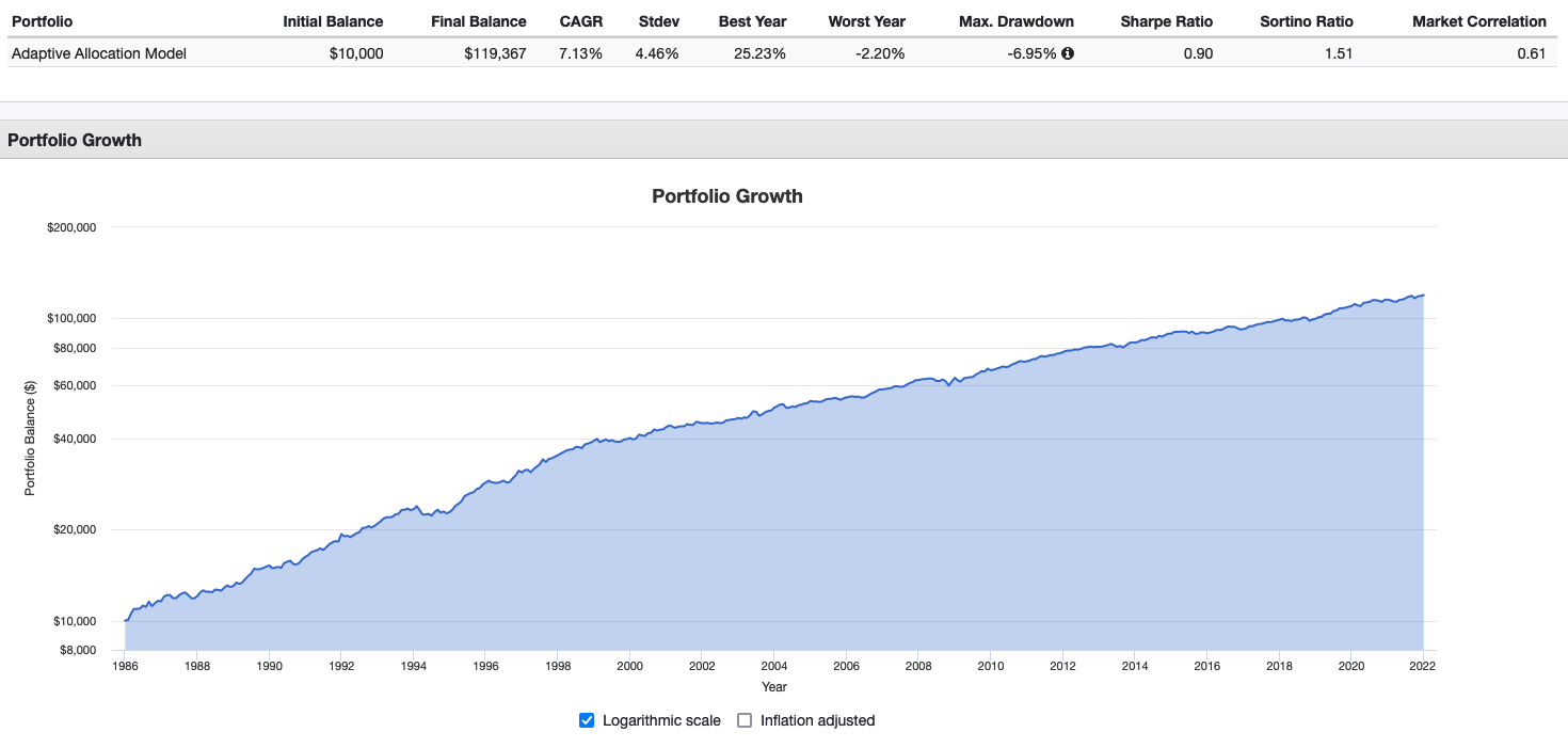
(This is a very simple mix of long-duration treasuries and stocks that you can replicate here).
But what does Risk Parity mean? Well, it’s one of these things that is simple in principle (but tricky in consequence, to which I’ll get later).
For a start: for RP, “volatility” is the chosen indicator of risk.
In general investing terms, a well-designed portfolio will have a mix of higher-risk and lower-risk assets. A conventional way to deal with these different risk profiles would be to have 60% of your assets in stocks, and 40% in bonds — the famous 60/40 portfolio.
Risk parity does it differently: it calculates the current volatility of each of your assets and allocates them accordingly.
Stocks can be very volatile/”risky” in some years (such as during the Great Financial Crisis, in 2008). That’s the time when you should own less of them and proportionately more treasuries. During other times (such as in 2021), stocks will be on a gentle, non-volatile upwards slope — so you might want to have 70% or even 80% of your investments in stocks.
An additional thing that Risk Parity does is acknowledge that all assets have inherent risks and inherent leverage. Corporations have various degrees of debt/leverage, and a government bond may be more or less risky (depending on the times, and on the economy, and on the country). A flexible risk allocation makes more sense than assuming, in a rather rigid way, that stocks are generally very risky and that all bonds are fine. Don’t rely on that rating agency that said things were Triple-A in late 2007; focus on the price action!
How to calculate your current Risk Parity allocation?
The details of the volatility-allocation formula used to be quite mathematical/arcane, but with all the financial web services available nowadays, this is no longer a problem for the numerically semi-stupid (as I happen to be). The above equity curve is that of a simple treasuries/stocks Risk Parity strategy that I made with the “adaptive allocation” tool of Portfoliovisualizer, and you can use it free of charge, too (as long as you don’t need real-time investment allocation data).
So, what went wrong after those 40 years of excellent performance?
Risk Parity looked like it could put no foot wrong. The above strategy had in the 35 years from 1986 to 2021 only one negative year.

It seemed to be able to ignore all the emotion and uproar of the financial markets, no matter whether it was the Crash of ‘87, The Latin American debt crisis, LTCM, the Dotcom Bubble’s bursting, the Great Financial Crisis of 2008, or the Covid Pandemic. Not to mention all the little crises, corrections, and bearish markets in between. So, as the years went by, ever more millions and millions got invested in Risk Parity funds.
However, RP’s Achilles heals were its reliance on the inverse relationship between stocks and treasuries, and its inability to go to cash in really bad times.
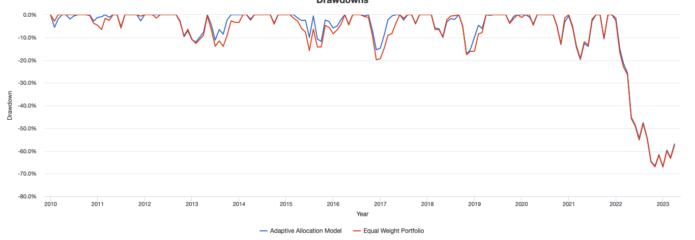
Normally, stocks are profitable in good times, and treasuries are successful compensators in bad times. However, in 2022, this inverse relationship went to pot. Both stocks and government bonds lost more than 15%, so (citing again the above simple strategy), this is what happened after 2021:

Moreover, Risk Parity strategies do not have a cash component, among other reasons because cash has no volatility. In the end, RP as we knew it could not deal with a situation in which most asset types were losing value at the same time. It had no safe “risk-off” space.
My proposition: add a moving average filter to our Risk Parity assets
Let’s start with a strategy that I quite enjoyed using until 2022: Varan’s 2-Asset Risk Parity. It employs leveraged ETFs: QLD (2x the Nasdaq technology index) and TMF (3x long-term treasury; its unleveraged equivalent is TLT).
From 2010 onwards, up to and including 2021, Varan’s strategy had a wonderful performance of CAGR 31.96%, and a maximum monthly drawdown of -19.74%. Sure, quite volatile, but very profitable!
But it all blew up in 2022, degrading its CAGR (up to end-March, 2023) to 20.76%, while its maximum drawdown rocketed to -66.89%, which sounds bad enough, but holy cow, look at this diagram:
The obvious response to such a damaging year would be to say: this is a broken approach, abandon ship!
However, after seeing its powerful performance in the first three months of 2023 of 30.07%, I wondered whether it might be salvageable. Which led to this experiment:
First new strategy: “Varan 2 RP+MA, Winner Takes All”
We continue using the risk parity strategy’s rules of monthly re-distributions, but in addition, sell TMF and/ or QLD in the months in which the price of these ETFs are below their 200-day moving averages. If TMF is below its 200-dma, then we buy to 100% QLD (the “winner”), and vice-versa. If both are below their 200-dma, we then go 100% to cash.
I assumed this might be somewhat effective because the moving averages would take us to cash for most of 2022. At the same time, I was expecting a big hit in CAGR — using moving averages as a filter usually acts like a kind of insurance against both big losses and great gains, which means you’re paying a premium.
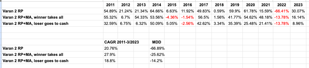
However, the results of this first tweak were better than I expected. CAGR 1/2011-3/2023 is now 27.9%, and the maximum monthly drawdown is -25.62%.
Second new strategy: “Varan 2 RP+MA, Loser Goes to Cash”
Depending on your preferences, this may be the best variant.
Here, we invest the selected assets according to the percentages that Risk Parity has calculated for us.
In other words: Say, in a given month TMF is under its 200-day moving average and therefore “out”. QLD in contrast is doing fine, and our RP algorithm says we should allocate 52% of our funds to it. So exactly this we do, and we sell all of the “loser” asset TMF, and with this money (which is 48% of our invested funds), we go to cash.
(And just as in the previous variant, we go 100% to cash when both TMF and QLD are “losers”).
Results: CAGR 18.8%, maximum monthly drawdown -14.2%.
This has the best risk-adjusted return: MAR = 1.32 vs 1.09.
If these strategies were just an element of a Talebesque barbell approach — where 10% of your funds are invested in a high-flyer strategy, and the rest in safe assets - then you’d go for the strategy with the highest absolute returns. Otherwise, of course, a better risk-adjusted return is always advisable.
Here’s the yearly data:
Good times, bad times
When do I hope this strategy is going to be effective?
When we have timing luck. A Nasdaq waterfall crash starting on the second trading day of the month is not something a monthly strategy deals with well. Soon, I will test a weekly strategy that would probably mitigate the greatest part of this caveat. That said, weekly strategies require a lot of futzing around with weekly rebalances…
When the markets are not see-sawing. Trend-following is not very effective when there is no real trend. Nonetheless, the original, unleveraged strategy performed reasonably well during the “trendless” years of 2001 and 2002, because it seldom happens that both stocks and treasuries are in a funk.
Risk parity won’t work if we get double-dip or triple-dip inflation that harms both stocks and bonds. In February 2022, our strategy took us out of the market — but only after a loss of 13.78% signaled “risk-off”. You don’t need many such episodes to get fed up.
Important disclaimer
Every strategy that intends to achieve a higher than 15% CAGR will blow up sooner or later. Common knowledge.
Only morons or suicidals use leverage on more than 5% of their investible funds.
There, I said it.
By the way, the theory looks good as well
The Trend is Our Friend: Risk Parity, Momentum and Trend Following in Global Asset Allocation
Combining Trend Following and Risk Parity across Asset Classes
Next steps?
I’ll test a weekly strategy.
And, I’ll test to see what happens to the simple strategy (from 1987 onwards), when Risk Parity is combined with Momentum.
You’ll write something in the comments section to let me know whether this has any merit, and if you think I should continue.
Thanks for reading!
Ah, and I forgot to say thanks for the post! Great read!
Martin, I'm contemplating your disclaimer on CAGR over 15% and "suicidal". :-)
I'd say in addition to looking at weekly in addition to monthly you might also look at adding a 50 day MA to your 200 day, and staying at monthly rebalances. Where both 50 and 200 must be positive, else sell/cash.
Looking at the returns in PV, it looks like the strategy provides an additional 4% or so CAGR over equal weights. The real issue I see is that the correlations between the two classes switched from somewhat uncorrelated to high correlated in 2022, and that coincides with a downturn on both (it wouldn't hurt if it was an uptrend on both). Maybe we should try to look at the trends of correlation as well?